Exact Spreading Resistance in Vertical Contacts to Anisotropic Thin Films
An exact field solution captures anisotropy, finite geometry, and interfacial resistivity in planar and cylindrical contacts.
Building an exact model for a finite anisotropic contact
Spreading resistance is the extra voltage drop created when current leaves a finite contact and redistributes into a larger conducting region. Classical expressions are compact and useful, but they usually assume isotropic transport, idealized geometry, or semi-infinite media.
Those assumptions become questionable for modern layered devices. A vertical contact to a thin MoS$_2$, WSe$_2$, graphite, or other van der Waals layer may have strong conductivity anisotropy, a finite channel width, nanometer-scale thickness, and a nonzero interfacial resistance.
Our published framework was developed to keep all of those ingredients in the same field solution.
The governing equation keeps the tensor physics
In each material region, the potential satisfies
$ \nabla\cdot\left(\boldsymbol{\sigma}\nabla\Phi\right)=0. $
The conductivity tensor is diagonal in the principal material directions, so the in-plane and out-of-plane conductivities can be specified independently.
For two stacked layers,
$ \boldsymbol{\rho}1= \operatorname{diag}\left(\rho{1,t},\rho_{1,z}\right), \qquad \boldsymbol{\rho}2= \operatorname{diag}\left(\rho{2,t},\rho_{2,z}\right). $
where (t) denotes the lateral coordinate and (z) the vertical direction.
The two regions are joined through a finite specific interfacial resistivity $\rho_i$, which permits a potential discontinuity proportional to the normal current density.
This boundary condition is important because the interface is not simply added after the field solution. A finite interface resistance can alter the way current spreads in the adjoining materials.
Cartesian and cylindrical contacts
The theory is derived for both planar and disk-shaped contacts.
In Cartesian geometry, a contact of half-width $a$ injects current into a lower region extending to a half-width (b>a). In cylindrical geometry, the same variables become the contact radius and surrounding device radius.
The total contact resistance can be decomposed conceptually as
\[R_c = R_s + R_{\mathrm{interface}} + R_1,\]where $R_s$ is the spreading resistance, $R_{\mathrm{interface}}$ is the interface contribution, and $R_1$ is the vertical resistance of the upper contact material.
This decomposition makes it possible to see which physical contribution dominates for a given geometry and material set.
Why exact geometry matters
A semi-infinite approximation cannot know when a real device edge is close to the contact.
If the peripheral boundary is far away and the lower layer is thick, the current has enough space to spread naturally. But when (b/a) becomes small or the film thickness is reduced, the boundaries constrain the current paths.
The exact solution captures those finite-size effects automatically because the device dimensions enter the field expansion and boundary conditions.
This is especially important in nanoscale contacts, where a contact radius, channel width and film thickness may differ by only one or two orders of magnitude rather than by many decades.
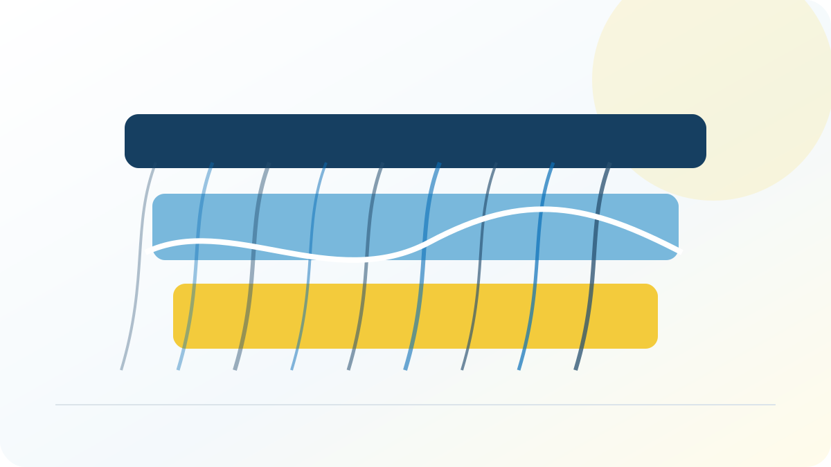
Anisotropy becomes a geometric transformation of the field
One useful way to interpret the mathematics is that anisotropy effectively stretches one coordinate relative to another.
When lateral resistivity is much smaller than vertical resistivity, equipotential contours spread much farther along the plane. The current density becomes correspondingly concentrated near the contact edges.
The exact field solution therefore connects a measurable terminal quantity — spreading resistance — to the spatial distribution that causes it.
That is an advantage over a purely lumped model.
Recovering familiar limiting cases
A good general model should reduce to known results when its extra physics is removed.
The framework recovers previously established isotropic finite-boundary solutions and the known single-layer anisotropic limit. In the wide-and-thick regime, it also approaches the classical diffusive (1/a) scaling used for spreading resistance.
These limits are valuable checks because they show that the exact anisotropic formulation extends rather than replaces the classical theory.
Why the model is useful experimentally
The field solution is not only intended for forward prediction.
Because the model explicitly includes $a$, $b$, $h_1$, $h_2$, $\rho_i$, and the anisotropic resistivities, it can be used to interpret experimental resistance data without folding geometry into an uncontrolled effective parameter.
That matters when extracting intrinsic transport properties. If an experiment lies outside the wide, thick, semi-infinite regime, fitting it with a simple (1/a) law can return a misleading in-plane or out-of-plane resistivity.
The exact model provides a physics-based alternative in which material anisotropy and actual device dimensions remain visible throughout the calculation.