How Grating Geometry Sets Frequency and Starting Current in Smith–Purcell Radiation
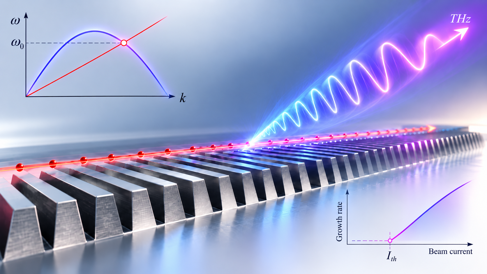
How groove height and width reshape the cold-tube dispersion, move the operating frequency, and ultimately control the threshold for coherent THz Smith–Purcell radiation.
Why grating geometry matters
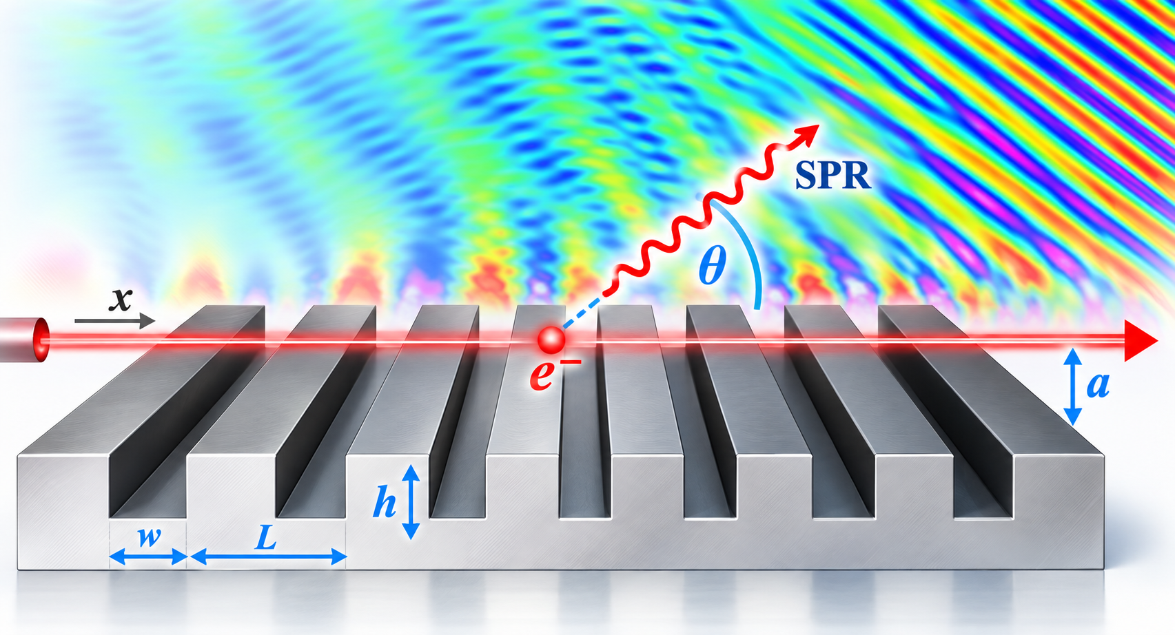
Smith–Purcell radiation (SPR) is produced when an electron beam moves close to a periodic metallic grating. The basic picture is simple: the moving electrons excite electromagnetic fields near the grating, and part of that interaction appears as radiation at a wavelength set by the beam velocity, the grating period, the diffraction order, and the observation angle [1,2].
The familiar Smith–Purcell relation is
\[\lambda = \frac{L}{n} \left( \frac{1}{\beta} - \cos\theta \right),\]where $L$ is the grating period, $n$ is the diffraction order, $\beta=v/c$ is the normalized beam velocity, and $\theta$ is the observation angle.
This equation is important, but it does not contain the groove height $h$ or groove width $w$. That can give the impression that these dimensions are secondary. In a coherent Smith–Purcell oscillator, they are not. The groove geometry changes the electromagnetic slow-wave mode supported by the grating, and this changes both the operating frequency and the strength of the beam–wave interaction [1,3,4].
In our published study, the grating period and electron-beam properties were kept fixed while $h$ and $w$ were varied. The starting current changed by orders of magnitude [1]. The central question was therefore not simply “what wavelength is radiated?” but rather:
How does the detailed grating geometry change the mode that the beam interacts with?
The answer begins with the cold-tube dispersion relation.
The cold-tube problem: first find the passive grating mode
“Cold tube” means that the electron beam is not yet included in the electromagnetic dispersion calculation. We first ask what surface mode the periodic metallic grating supports by itself.
The analysis uses normalized quantities
\[\bar{\omega}=\frac{\omega L}{c}, \qquad \bar{k}=kL, \qquad \bar{W}=\frac{w}{L}, \qquad \bar{H}=\frac{h}{L}.\]For the rectangular grating model used in the paper, the cold-tube surface-mode relation is [1]
\[\frac{\cot\!\left(\bar{\omega}\bar{H}\right)} {\bar{\omega}\bar{H}} - \sum_{n=-\infty}^{\infty} \left( \frac{\sin\theta_n}{\theta_n} \right)^2 \frac{\bar{W}} {\gamma_n\bar{H}} = 0,\]with
\[\theta_n=\frac{P_n\bar{W}}{2}, \qquad P_n=\bar{k}+2n\pi,\]and
\[\gamma_n= \sqrt{P_n^2-\bar{\omega}^2}.\]The physical idea behind this equation is easier than the expression itself. The field inside each groove is matched to the Floquet harmonics above the periodic grating. The groove width, groove height, and period therefore enter directly into the allowed surface-wave dispersion [1,5].
The paper used the dominant TEM-like groove mode for this calculation. A sufficiently large number of spatial harmonics was retained numerically to ensure convergence [1].
The beam line selects the operating point
After the cold dispersion curve is known, the electron beam is introduced only as a synchronism line. For a beam with velocity $v_0$,
\[\omega = kv_0.\]In normalized form,
\[\bar{\omega} = \beta_0\bar{k},\]where
\[\beta_0=\frac{v_0}{c}.\]For the 50-keV beam used in the paper,
\[\beta_0=0.4126.\]The intersection of this beam line with the cold-tube dispersion curve gives the evanescent surface-mode operating frequency $f_{\mathrm{ev}}$ [1].
This is the first key design result: even with fixed beam energy and fixed grating period, changing $h$ or $w$ moves the intersection point. Therefore, groove geometry changes the operating frequency.
The coherent SPR of interest in the study occurs at the corresponding harmonic of the evanescent mode [1].
Why deeper or wider grooves lower the operating frequency
The numerical sweeps in the paper show a clear trend. As either the groove height $h$ or groove width $w$ increases, the operating frequency generally decreases, while the corresponding evanescent wavelength increases [1].
The reason is visible directly in the cold-tube dispersion curve. Increasing the groove dimensions changes the upper band edge. The band edge becomes lower and more rounded, so the same electron beam line intersects the curve at a smaller frequency.
That gives a practical tuning mechanism. Two gratings can have the same period $L$ and use the same beam energy, yet operate at different frequencies because the groove dimensions are different.
This is why the basic Smith–Purcell wavelength equation is not a complete device-design rule. It captures the radiation kinematics, while the cold-tube dispersion captures the actual slow-wave mode supported by the structure [1,3].
Geometry can even change the wave direction
The slope of the dispersion curve gives the group velocity,
\[v_g = \frac{d\omega}{dk}.\]For many of the geometries in the paper, the slope at the operating point is negative, which is characteristic of backward-wave behavior.
However, for deeper grooves around
\[h=120\text{–}200~\mu\mathrm{m},\]the slope becomes positive in the reported sweep [1].
That means a purely geometric modification can move the beam–grating interaction from a backward-wave-like region to a forward-wave-like region, even though the beam energy and grating period remain unchanged.
This is a strong reminder that $h$ and $w$ do not make only small corrections. They can change the qualitative electromagnetic character of the interaction.
The same geometry also changes spatial growth
Cold-tube dispersion tells us where the beam and grating can interact. It does not yet tell us how strongly the coupled wave will grow.
That requires the hot-tube model, where the beam dynamics are included self-consistently. The hot solution gives a complex wavenumber
\[k=k_r+jk_i.\]For the field convention used in the paper,
\[E(x,t)\propto e^{-j\omega t+jkx},\]so
\[E(x,t) \propto e^{-j\omega t+jk_r x} e^{-k_i x}.\]If $k_i<0$, the field grows with distance. The spatial growth rate is therefore
\[g_s=-k_i.\]The important result is that the growth rate also depends strongly on $h$ and $w$ [1].
For the parameter sweeps reported in the paper, strong growth occurs near groove heights around
\[h\approx100\text{–}120~\mu\mathrm{m},\]for the fixed-width sweep, and near
\[w\approx80~\mu\mathrm{m},\]for the fixed-height sweep [1].
These high-growth points occur when the operating point approaches the upper band edge of the cold dispersion curve. Band-edge regions are known to be particularly sensitive to beam-driven instability [6].
Why this matters for starting current
The starting current is the minimum dc beam current required for coherent oscillation to build. Below this current, the beam may still interact with the grating, but the modulation is not strong enough to produce sustained electron bunching and coherent radiation [1,4].
The paper compared the calculated spatial growth rate with starting currents obtained independently from particle-in-cell simulations using a 35-period grating [1,3].
The result is very clear: the geometry dependence of the starting current closely follows the geometry dependence of the spatial growth rate.
Geometries with larger $-k_i$ require lower starting current.
This means that groove optimization can be organized as a two-step physics problem:
- use the cold-tube dispersion to find the operating frequency;
- use the hot-tube growth rate to find the geometry that reaches coherent oscillation most easily.
This is much more efficient than using a full PIC starting-current search at every point in a large geometry sweep.
A practical optimization workflow
A useful design workflow is therefore:
1. Choose the beam energy and grating period
These set the basic beam line and periodic scale.
2. Sweep groove height and width
For each pair $(h,w)$, calculate the cold-tube dispersion.
3. Find the beam–mode intersection
Use
\[\bar{\omega}=\beta_0\bar{k}\]to determine $f_{\mathrm{ev}}$.
4. Check the desired radiation frequency
Reject geometries whose operating point is outside the target range.
5. Solve the hot-tube dispersion
Obtain
\[k=k_r+jk_i.\]6. Rank the remaining geometries by $-k_i$
Larger $-k_i$ means stronger spatial amplification.
7. Use PIC only for final verification
PIC is then applied to a small set of promising designs rather than the entire parameter space.
This strategy keeps the physical meaning visible at every step. Geometry first changes the passive mode, and the changed mode then modifies the beam-driven growth.
The main design lesson
The most important lesson is simple:
A Smith–Purcell grating is not defined only by its period.
The groove width and height reshape the slow-wave dispersion, move the operating frequency, change the group velocity, change the spatial growth rate, and ultimately change the starting current.
For THz device design, the useful geometry is therefore not simply the one that satisfies the Smith–Purcell wavelength relation. Similar slow-wave-structure considerations and three-dimensional beam requirements are also important when the design moves toward a practical device [7,8]. It is the geometry that places the desired frequency at a strong beam–wave operating point with sufficiently large spatial gain.
That is why cold-tube and hot-tube dispersion should be used together [1]. The first tells us where the device operates. The second tells us how strongly it can grow.
References
- M. A. Faisal and P. Zhang, “Grating Optimization for Smith–Purcell Radiation: Direct Correlation Between Spatial Growth Rate and Starting Current,” IEEE Transactions on Electron Devices, vol. 70, pp. 2860–2863, 2023. DOI: 10.1109/TED.2022.3208846.
- S. J. Smith and E. M. Purcell, “Visible Light From Localized Surface Charges Moving Across a Grating,” Physical Review, vol. 92, p. 1069, 1953. DOI: 10.1103/PhysRev.92.1069.
- P. Zhang, L. K. Ang, and A. Gover, “Enhancement of Coherent Smith–Purcell Radiation at Terahertz Frequency by Optimized Grating, Prebunched Beams, and Open Cavity,” Physical Review Special Topics – Accelerators and Beams, vol. 18, 020702, 2015. DOI: 10.1103/PhysRevSTAB.18.020702.
- V. Kumar and K.-J. Kim, “Analysis of Smith–Purcell Free-Electron Lasers,” Physical Review E, vol. 73, 026501, 2006. DOI: 10.1103/PhysRevE.73.026501.
- H. P. Freund and T. M. Abu-Elfadl, “Linearized Field Theory of a Smith–Purcell Traveling Wave Tube,” IEEE Transactions on Plasma Science, vol. 32, pp. 1015–1027, 2004. DOI: 10.1109/TPS.2004.827612.
- D. M. H. Hung et al., “Absolute Instability Near the Band Edge of Traveling-Wave Amplifiers,” Physical Review Letters, vol. 115, 124801, 2015. DOI: 10.1103/PhysRevLett.115.124801.
- S. C. Yurt et al., “Similarity of Properties of Metamaterial Slow-Wave Structures and Metallic Periodic Structures,” IEEE Transactions on Plasma Science, vol. 44, pp. 1280–1286, 2016. DOI: 10.1109/TPS.2016.2535305.
- K.-J. Kim and V. Kumar, “Electron Beam Requirements for a Three-Dimensional Smith–Purcell Backward-Wave Oscillator for Intense Terahertz Radiation,” Physical Review Special Topics – Accelerators and Beams, vol. 10, 080702, 2007. DOI: 10.1103/PhysRevSTAB.10.080702.