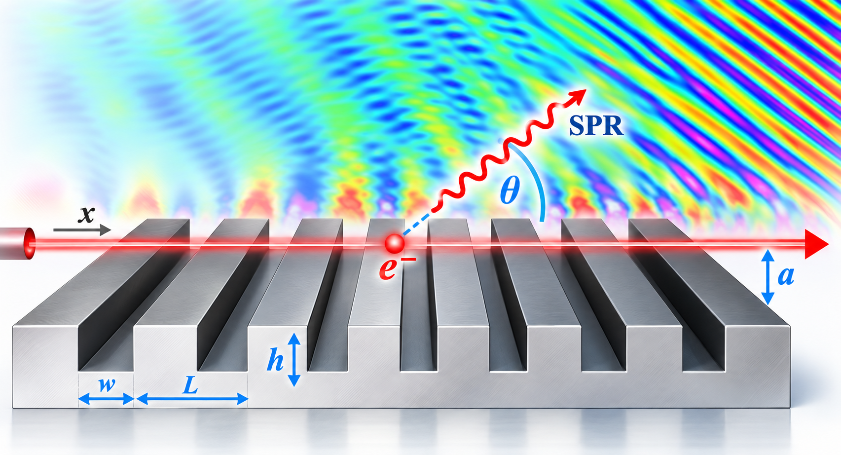
Cold- to Hot-Tube Dispersion Derivation: A Tutorial on Smith-Purcell Radiation Growth Rate
A step-by-step tutorial on deriving cold- and hot-tube dispersion relations for Smith–Purcell radiation, calculating spatial growth rates, and relating them to the starting current from PIC simulation.
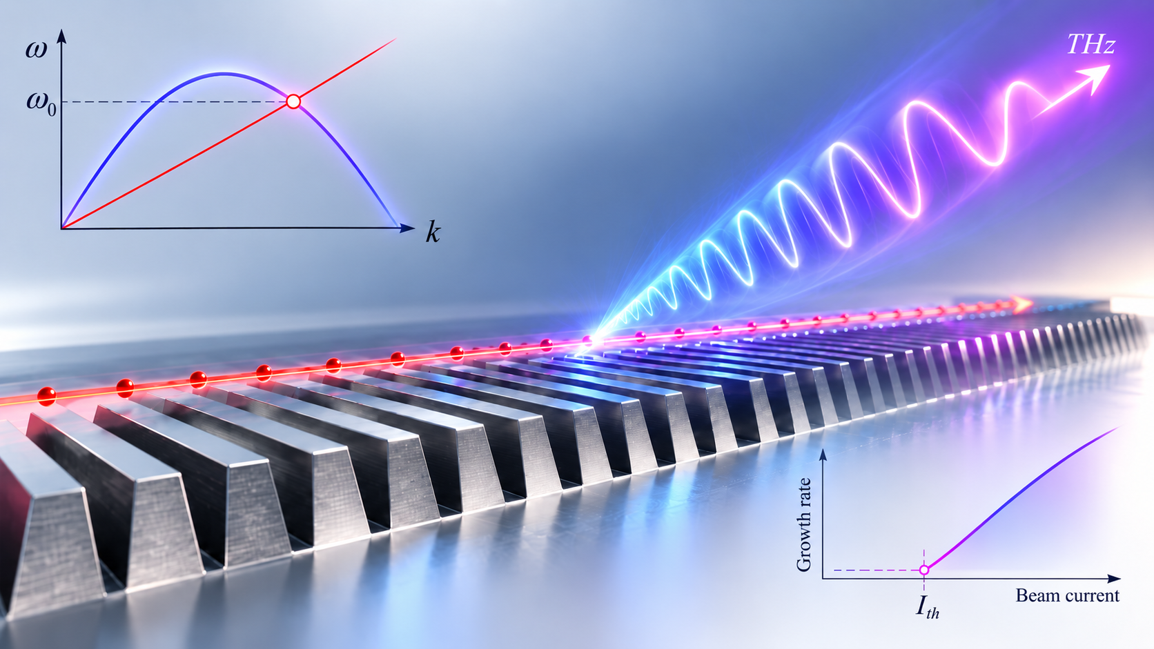
Why starting current is really a growth problem
A coherent Smith–Purcell oscillator does not begin at full strength as soon as electrons pass over a grating. The electron beam first interacts with the evanescent slow wave supported by the periodic metal structure. That interaction creates a small velocity modulation. After some distance, the velocity modulation becomes density modulation, or electron bunching. When the bunching becomes strong enough, the beam can transfer coherent energy to the electromagnetic mode and the oscillation grows [1,3,4].
The minimum dc beam current required for this process to build into coherent radiation is the starting current.
A direct way to find it is to repeat particle-in-cell (PIC) simulations at many beam currents and identify the threshold at which a sustained coherent field appears. That method is powerful, but it is expensive when many grating geometries must be tested.
Our published work showed that the same threshold trend can be predicted from the spatial growth rate calculated from the hot-tube dispersion relation [1].
This article develops that connection from the beginning: fields, boundary matching, beam perturbation, hot-tube dispersion, complex roots, spatial growth, and finally the comparison with PIC.
Researcher roadmap: first solve the electromagnetic fields in each region, then match those fields at the grating boundary, then add the electron-beam response, and finally solve the resulting dispersion equation for a complex wavenumber.
What you will get from this article?
By the end, you should be able to identify what is being solved at each stage:
- Field problem: write Maxwell-consistent fields in the groove and above the grating.
- Boundary problem: match tangential fields to obtain the passive, or cold-tube, dispersion.
- Beam problem: linearize the electron continuity and momentum equations.
- Coupled problem: insert the beam response into the field matching to obtain the hot-tube dispersion.
- Root problem: solve the hot-tube equation for $k=k_r+jk_i$ at a real operating frequency.
- Design problem: use $-k_i$ to estimate which geometry should have the lowest starting current.
Step 1: begin with Maxwell’s equations
For the two-dimensional $x$-$y$ model, the relevant TM-like field set can be written using $H_z$, $E_x$, and $E_y$. With harmonic time dependence $e^{-i\omega t}$, Maxwell’s equations are
\[\nabla\times\mathbf{E} = i\omega\mu_0\mathbf{H},\]and
\[\nabla\times\mathbf{H} = \mathbf{J} - i\omega\epsilon_0\mathbf{E}.\]Before the electron beam is introduced, $\mathbf{J}=0$ in the vacuum regions. Once the beam is added, its ac current becomes part of the second equation.
The main task is to first solve the passive grating fields. We obtain the cold-tube dispersion from the two-region problem, then add the beam and construct the three-region hot-tube problem.
Step 2: write the cold-tube fields in the two regions
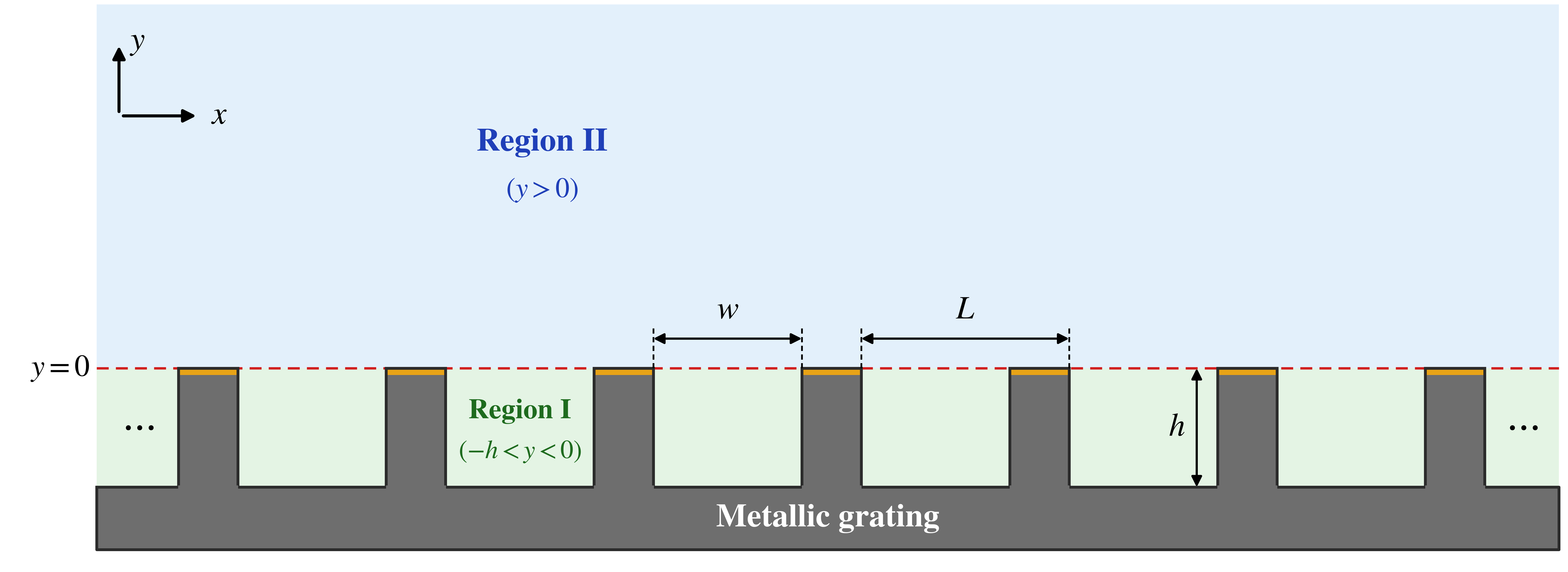
For the cold-tube problem, the electron beam is not yet allowed to load the electromagnetic mode. The structure therefore needs only two electromagnetic regions: Region I inside a groove and Region II in the vacuum above the grating. The dispersion relation is obtained by solving Maxwell’s equations in these two regions and matching the tangential fields at the grating surface [1,5,6].
Region I: inside a groove
Let the groove occupy
\[-h<y<0.\]Using the groove-mode form employed in the field-matching treatment [5], the fields can be written as
\[H_{1,z}(x,y,t) = \bar{H}_{1z,0} \frac{\cosh\!\left[k_0(y+h)\right]} {\sinh(k_0 h)} e^{-i\omega t},\]and
\[E_{1,x}(x,y,t) = \bar{E}_{1x,0} \frac{\sinh\!\left[k_0(y+h)\right]} {\cosh(k_0 h)} e^{-i\omega t}.\]The amplitude factors absorb the normalization used in the full modal solution. The important feature here is the explicit groove-depth dependence and the fact that the tangential electric field satisfies the conducting boundary at the groove bottom.
Region II: vacuum above the grating
For the cold-tube problem,
\[0<y<\infty.\]Because the grating is periodic along $x$, the vacuum field is expanded in Floquet harmonics. Since this region extends to $y\rightarrow\infty$, only the decaying solution is physically allowed:
\[H_{2,z}(x,y,t) = \sum_{p=-\infty}^{\infty} H_{2,p} e^{-\alpha_p y} e^{i\beta_p x} e^{-i\omega t},\] \[E_{2,x}(x,y,t) = \sum_{p=-\infty}^{\infty} \left( -i\frac{\alpha_p}{\omega\epsilon_0} \right) H_{2,p} e^{-\alpha_p y} e^{i\beta_p x} e^{-i\omega t},\]and
\[E_{2,y}(x,y,t) = \sum_{p=-\infty}^{\infty} \frac{\beta_p}{\epsilon_0\omega} H_{2,p} e^{-\alpha_p y} e^{i\beta_p x} e^{-i\omega t}.\]Here,
\[\beta_p = k+\frac{2\pi p}{L},\]and
\[\alpha_p = \sqrt{\beta_p^2-\left(\frac{\omega}{c}\right)^2}.\]For an evanescent surface harmonic we choose the branch with
\[\operatorname{Re}(\alpha_p)>0,\]so the field decays away from the grating. There is no growing term $e^{+\alpha_p y}$ in the cold-tube Region II, because such a term would diverge as $y\rightarrow\infty$.
This two-region field picture is the one used to obtain the passive grating dispersion. The third field region appears only after the electron beam is introduced in the hot-tube problem.
Step 3: match the fields at the grating surface
Now the two regional solutions are connected at $y=0$.
Over the groove opening, the tangential fields are continuous:
\[H_{1,z}=H_{2,z},\]and
\[E_{1,x}=E_{2,x}.\]Over the metallic part of the grating surface, the tangential electric field must vanish:
\[E_{2,x}=0.\]Because Region II is written as a Floquet series, these conditions are projected over one grating period. This converts the boundary-matching problem into algebraic relations among the groove amplitude and the harmonic amplitudes $H_{2,p}$ [1,5,6].
After eliminating the amplitudes, the passive or cold-tube dispersion relation is obtained.
Using the normalized quantities
\[\bar{\omega}=\frac{\omega L}{c}, \qquad \bar{k}=kL, \qquad \bar{W}=\frac{w}{L}, \qquad \bar{H}=\frac{h}{L},\]define
\[P_n=\bar{k}+2n\pi,\] \[\theta_n=\frac{P_n\bar{W}}{2},\]and
\[\gamma_n= \sqrt{P_n^2-\bar{\omega}^2}.\]The cold-tube relation can then be written [1]
\[\frac{\cot(\bar{\omega}\bar{H})} {\bar{\omega}\bar{H}} - \sum_{n=-\infty}^{\infty} \left( \frac{\sin\theta_n}{\theta_n} \right)^2 \frac{\bar{W}} {\gamma_n\bar{H}} = 0.\]This equation answers the first design question:
What electromagnetic surface mode does the grating support before beam loading is included?
Our later two-layer analysis follows the same logic: define the passive field regions first, apply the interface conditions, and then add the beam-loaded regions needed for the hot-tube problem [5].
Step 4: use the beam line to select the operating frequency
The electron beam has axial velocity $v_0$. Its synchronism line is
\[\omega=kv_0.\]In normalized form,
\[\bar{\omega} = \beta_0\bar{k},\]where
\[\beta_0=\frac{v_0}{c}.\]The intersection of this beam line with the cold-tube dispersion curve gives the evanescent-wave operating frequency used for the hot-tube calculation [1].
For the 50-keV beam used in the published study,
\[\beta_0=0.4126.\]At this stage, the beam is only selecting the operating point. It has not yet modified the dispersion.
Step 5: introduce the hot-tube field regions
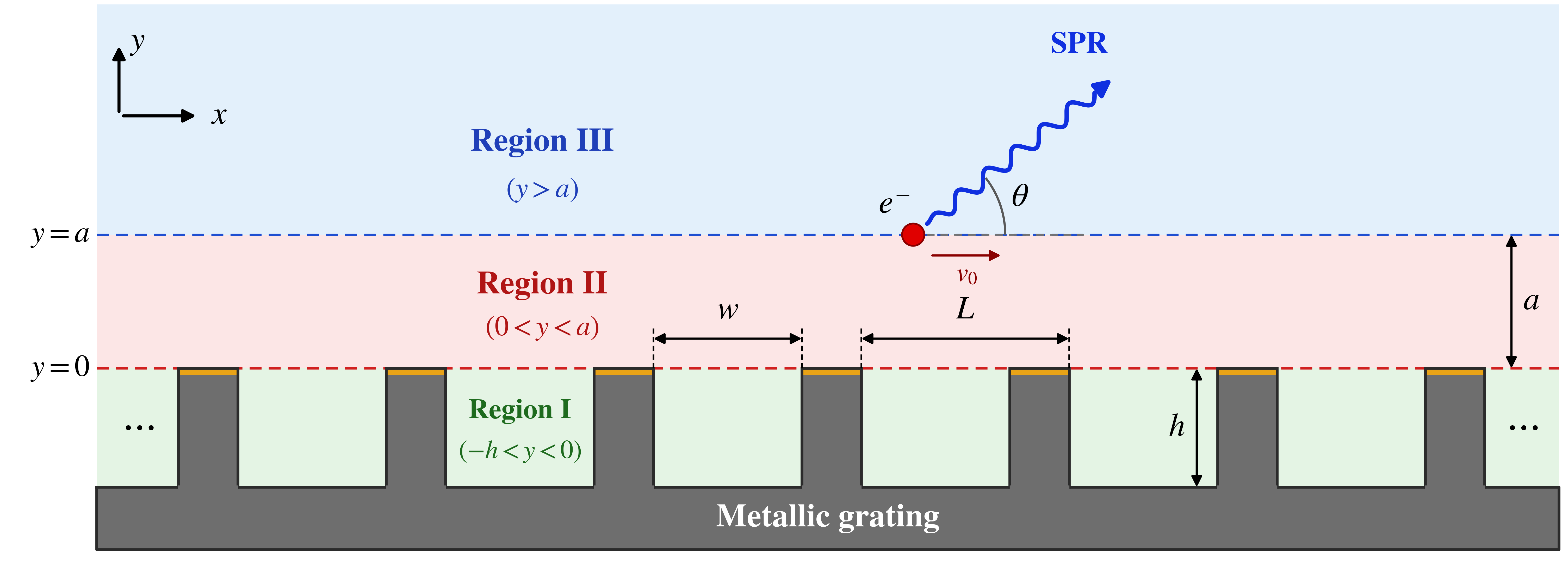
The cold-tube calculation treated the whole space above the grating as one decaying vacuum region. Once the electron beam is placed at
\[y=a,\]that vacuum region must be split at the beam plane.
The hot-tube field problem therefore uses three regions:
- Region I: groove, $-h<y<0$;
- Region II: vacuum between the grating and beam, $0<y<a$;
- Region III: vacuum above the beam, $y>a$.
Region I keeps the same groove field used in the cold-tube problem. The change occurs above the grating.
Hot-tube Region II: between the grating and the beam
Because Region II is now bounded by the grating at $y=0$ and the beam at $y=a$, both exponential solutions are needed:
\[H_{2,z}(x,y,t) = \sum_{p=-\infty}^{\infty} \left( H_{2z-,p}e^{-\alpha_p y} + H_{2z+,p}e^{\alpha_p y} \right) e^{i\beta_p x} e^{-i\omega t},\] \[E_{2,x}(x,y,t) = \sum_{p=-\infty}^{\infty} \left( -i\frac{\alpha_p}{\omega\epsilon_0} \right) \left( H_{2z-,p}e^{-\alpha_p y} - H_{2z+,p}e^{\alpha_p y} \right) e^{i\beta_p x} e^{-i\omega t},\]and
\[E_{2,y}(x,y,t) = \sum_{p=-\infty}^{\infty} \frac{\beta_p}{\epsilon_0\omega} \left( H_{2z-,p}e^{-\alpha_p y} + H_{2z+,p}e^{\alpha_p y} \right) e^{i\beta_p x} e^{-i\omega t}.\]The $e^{+\alpha_p y}$ term is allowed here because Region II is finite: it ends at the beam plane rather than extending to infinity.
Hot-tube Region III: above the beam
For
\[y>a,\]the field must again decay as $y\rightarrow\infty$. Therefore,
\[H_{3,z}(x,y,t) = \sum_{p=-\infty}^{\infty} H_{3,p} e^{-\alpha_p(y-a)} e^{i\beta_p x} e^{-i\omega t},\] \[E_{3,x}(x,y,t) = \sum_{p=-\infty}^{\infty} \left( -i\frac{\alpha_p}{\omega\epsilon_0} \right) H_{3,p} e^{-\alpha_p(y-a)} e^{i\beta_p x} e^{-i\omega t},\]and
\[E_{3,y}(x,y,t) = \sum_{p=-\infty}^{\infty} \frac{\beta_p}{\epsilon_0\omega} H_{3,p} e^{-\alpha_p(y-a)} e^{i\beta_p x} e^{-i\omega t}.\]At the beam plane, the tangential electric field is matched across $y=a$, while the ac beam current supplies the corresponding magnetic-field discontinuity. The next steps derive that beam response from the continuity and momentum equations [1,2,5,8].
Step 6: perturb the electron beam
Now include the beam dynamically.
Let the equilibrium electron density and velocity be $n_0$ and $v_0$. Write the beam variables as
\[n=n_0+n_1,\]and
\[v=v_0+v_1,\]with the small-signal conditions
\[\lvert n_1\rvert\ll n_0, \qquad \lvert v_1\rvert\ll v_0.\]Using $\lvert\cdot\rvert$ instead of vertical-bar characters also avoids Markdown interpreting the equation as a table.
The unperturbed beam current density is
\[J_0=-e n_0v_0.\]The purpose of the hot-tube model is to find how the small ac quantities $n_1$ and $v_1$ respond to the electromagnetic field and then feed back into Maxwell’s equations. This is the standard small-signal AC space-charge framework used in electron–circuit theory [2,8].
Step 7: linearize the beam continuity equation
Charge conservation gives
\[\frac{\partial n}{\partial t} + \frac{\partial(nv)}{\partial x} = 0.\]Substitute
\[n=n_0+n_1, \qquad v=v_0+v_1,\]and neglect second-order terms such as $n_1v_1$. The result is
\[\frac{\partial n_1}{\partial t} + v_0 \frac{\partial n_1}{\partial x} + n_0 \frac{\partial v_1}{\partial x} = 0.\]Assume the perturbations vary as
\[e^{-i\omega t+ikx}.\]Then
\[\frac{\partial}{\partial t}\rightarrow-i\omega, \qquad \frac{\partial}{\partial x}\rightarrow ik.\]Therefore,
\[-i(\omega-kv_0)n_1 + ikn_0v_1 = 0,\]which gives
\[n_1 = \frac{k n_0} {\omega-kv_0} v_1.\]This already reveals the importance of synchronism. The beam response becomes strong when
\[\omega\approx kv_0.\]Step 8: linearize the electron equation of motion
For the axial ac velocity, the linearized momentum equation is
\[m \left( \frac{\partial}{\partial t} + v_0 \frac{\partial}{\partial x} \right) v_1 = -eE_1.\]Using the same harmonic dependence gives
\[-im(\omega-kv_0)v_1 = -eE_1.\]Hence,
\[v_1 = -\frac{i e} {m(\omega-kv_0)} E_1.\]Substitute this into the continuity result:
\[n_1 = -\frac{i ekn_0} {m(\omega-kv_0)^2} E_1.\]The ac current is
\[J_1 = -e(n_0v_1+v_0n_1).\]The important part is the resonant factor
\[\frac{1} {(\omega-kv_0)^2}.\]It is the mathematical signature of strong beam response near synchronism [2,8].
Step 9: convert the beam response into the hot-tube coupling factor
The beam plasma frequency is
\[\omega_p = \sqrt{ \frac{e^2n_0} {m\epsilon_0} }.\]For the sheet-beam model used in the paper, beam thickness $\tau$ enters through
\[\omega_a^2 = \omega_p^2\tau.\]Define
\[\bar{\omega}_a = \frac{\omega_a L^{1/2}}{c}.\]The normalized beam–grating distance is
\[\bar{A} = \frac{a}{L}.\]For the $n$th spatial harmonic, the beam response enters through [1]
\[\Psi = \frac{ \bar{\omega}_a^2\gamma_n }{ (\bar{\omega}-P_n\beta_0)^2 }.\]The beam modifies the corresponding harmonic through
\[U_n = \frac{ 1- \Psi\cosh(\gamma_n\bar{A})/e^{\gamma_n\bar{A}} }{ 1- \Psi\sinh(\gamma_n\bar{A})/e^{\gamma_n\bar{A}} }.\]This form makes two pieces of physics visible.
First, the denominator
\[(\bar{\omega}-P_n\beta_0)^2\]contains beam synchronism.
Second, the factors involving $\gamma_n\bar{A}$ show why the beam must remain close to the grating: the surface field is evanescent, so coupling weakens with separation [1].
The same region-by-region field construction and beam-loading idea is developed more generally for a two-layer grating in our 2025 IEEE Transactions on Plasma Science paper [5].
Step 10: obtain the final hot-tube dispersion relation
After the beam response is inserted into the boundary-matching system, the final hot-tube relation becomes [1]
\[f(\bar{k},\bar{\omega}) \equiv \frac{ \cot(\bar{\omega}\bar{H}) }{ \bar{\omega}\bar{H} } - \sum_{n=-\infty}^{\infty} U_n \left( \frac{\sin\theta_n}{\theta_n} \right)^2 \frac{\bar{W}} {\gamma_n\bar{H}} = 0.\]Compare this with the cold-tube equation. The electromagnetic structure is similar, but now each spatial harmonic carries the beam-loading factor $U_n$.
That is the central mathematical step:
Cold tube: geometry determines the passive mode.
Hot tube: geometry and beam dynamics determine the coupled mode.
How do I solve the hot-tube equation numerically?
A practical workflow is:
- Solve the cold-tube dispersion first.
- Use the beam-line intersection to choose a real operating frequency $\bar{\omega}$.
- Select a harmonic truncation, for example $-N\le n\le N$.
- For a trial complex $\bar{k}$, evaluate $P_n$, $\gamma_n$, $\theta_n$, $\Psi$, $U_n$, and then $f(\bar{k},\bar{\omega})$.
- Solve the two real equations
for
\[\bar{k} = \bar{k}_r+i\bar{k}_i.\]- Use several initial guesses because multiple roots can exist.
- Retain the physically relevant root and repeat with larger $N$ to verify convergence.
- Sweep $h$, $w$, beam current, or beam height only after the root solver is stable.
A useful numerical check is to plot
\[\log_{10}\lvert f(\bar{k},\bar{\omega})\rvert\]over the complex-$k$ plane. Local minima provide good initial guesses for a Newton, secant, or two-dimensional root solver.
Step 11: interpret the complex wavenumber
At the selected real operating frequency, solve the hot-tube equation for
\[k=k_r+ik_i.\]The field varies as
\[E(x,t) \propto e^{-i\omega t+ikx}.\]Substituting the complex wavenumber,
\[E(x,t) \propto e^{-i\omega t} e^{ik_r x} e^{-k_i x}.\]Therefore,
- $k_i>0$ gives spatial decay;
- $k_i<0$ gives spatial growth.
The spatial growth rate is
\[g_s=-k_i.\]For one example in the paper,
\[w=60~\mu\mathrm{m}, \qquad h=40~\mu\mathrm{m},\]the normalized growing root is approximately
\[\bar{k}_r=4.3289, \qquad \bar{k}_i=-0.041.\]The negative imaginary part identifies the growing branch [1].
Why the hot-tube real part shifts
The real part of the hot-tube wavenumber is slightly different from the cold-tube beam-line intersection.
This is beam loading. Once the electron beam is allowed to respond dynamically, it perturbs the electromagnetic mode and slightly detunes the real propagation constant [1,8].
The shift in $k_r$ is physically meaningful, but for starting-current optimization the most important quantity is $k_i$, because it controls spatial amplification.
Where the strongest growth occurs
The 2023 paper swept groove geometry while keeping the other parameters fixed [1].
For
\[w=60~\mu\mathrm{m},\]the strongest growth occurred near
\[h\approx100\text{–}120~\mu\mathrm{m}.\]For
\[h=100~\mu\mathrm{m},\]the strongest growth occurred near
\[w\approx80~\mu\mathrm{m}.\]These operating points lie near the upper band edge of the cold-tube dispersion curve [1].
Band-edge regions can be especially susceptible to beam-driven instability, which provides a useful physical interpretation for the growth maximum [7].
Step 12: compare the growth rate with PIC starting current
Now comes the device-level test.
The paper compared
\[-\bar{k}_i\]from the hot-tube dispersion with the starting current obtained independently from PIC simulations [1,3,4].
The PIC model used a 35-period grating with the same basic beam and geometric parameters.
The result is the key finding:
When the spatial growth rate increases, the starting current decreases.
This agreement is valuable because the two calculations are fundamentally different.
The hot-tube model is a linear frequency-domain calculation.
PIC follows the nonlinear particle and field evolution in time.
Yet both show nearly the same dependence on groove geometry [1].
Why the correlation is exponential
For coherent radiation, the power scales approximately as
\[P \propto E^2 \propto N^2 \propto I^2,\]where $N$ is the number of coherently bunched electrons and $I$ is beam current [1,3].
Therefore, at the scaling level,
\[E\propto I.\]A spatially growing mode is amplified over interaction length $L_G$ as
\[E \propto e^{\lvert k_i\rvert L_G}.\]Combining the two relations gives
\[e^{\lvert k_i\rvert L_G} \propto I.\]This explains why the spatial-growth curve and the logarithm of the starting-current curve follow one another so closely [1].
The relation is a scaling argument, not a full nonlinear saturation model. Its value is that it explains why a linear hot-tube calculation can predict a nonlinear threshold trend.
Why this is useful for a new design
Suppose you want to optimize a new Smith–Purcell structure.
A brute-force approach would be:
- choose a geometry;
- build the PIC model;
- sweep beam current;
- find the starting current;
- repeat for every geometry.
That quickly becomes expensive.
A dispersion-guided approach is more efficient:
- derive or compute the cold-tube dispersion;
- locate the beam-synchronous operating frequency;
- add the beam equations;
- solve the hot-tube relation;
- extract the growing root;
- map $-\operatorname{Im}(k)$ over geometry;
- reserve PIC for the best candidates.
Our 2025 two-layer work uses the same basic philosophy for a more complicated structure: the fields are written in multiple regions, matched at all interfaces, and then used to determine how the additional layer changes the cold operating point and hot spatial growth [5].
This is why learning the derivation is useful beyond one grating geometry. The field expansion → boundary matching → beam response → complex root workflow can be reused for many linear free-electron slow-wave devices.
The physical picture in one sentence
The full derivation can be summarized as
geometry defines the fields → boundary matching defines the passive mode → the electron beam loads that mode → the complex hot-tube root gives spatial growth → spatial growth predicts the beam-current threshold.
That is the practical meaning of the imaginary wavenumber. It connects electromagnetic field theory directly to an experimentally relevant device quantity: the current required to start coherent radiation.
References
-
M. A. Faisal and P. Zhang, “Grating Optimization for Smith–Purcell Radiation: Direct Correlation Between Spatial Growth Rate and Starting Current,” IEEE Transactions on Electron Devices, vol. 70, no. 6, pp. 2860–2863, 2023. DOI: 10.1109/TED.2022.3208846 ↗
-
Y. Y. Lau and D. Chernin, “A Review of the AC Space-Charge Effect in Electron–Circuit Interactions,” Physics of Fluids B: Plasma Physics, vol. 4, no. 11, pp. 3473–3497, 1992. DOI: 10.1063/1.860356 ↗
-
P. Zhang, L. K. Ang, and A. Gover, “Enhancement of Coherent Smith–Purcell Radiation at Terahertz Frequency by Optimized Grating, Prebunched Beams, and Open Cavity,” Physical Review Special Topics – Accelerators and Beams, vol. 18, 020702, 2015. DOI: 10.1103/PhysRevSTAB.18.020702 ↗
-
D. Li et al., “Growth Rate and Start Current in Smith–Purcell Free-Electron Lasers,” Applied Physics Letters, vol. 100, 191101, 2012. DOI: 10.1063/1.4711803 ↗
-
M. A. Faisal and P. Zhang, “Parametric Analysis on Enhancement of THz Smith–Purcell Radiation by Two-Layer Grating Structure,” IEEE Transactions on Plasma Science, vol. 53, no. 6, pp. 1170–1185, 2025. DOI: 10.1109/TPS.2025.3567163 ↗
-
H. P. Freund and T. M. Abu-Elfadl, “Linearized Field Theory of a Smith–Purcell Traveling Wave Tube,” IEEE Transactions on Plasma Science, vol. 32, no. 3, pp. 1015–1027, 2004. DOI: 10.1109/TPS.2004.827612 ↗
-
D. M. H. Hung et al., “Absolute Instability Near the Band Edge of Traveling-Wave Amplifiers,” Physical Review Letters, vol. 115, 124801, 2015. DOI: 10.1103/PhysRevLett.115.124801 ↗
-
P. Wong, P. Zhang, and J. Luginsland, “Recent Theory of Traveling-Wave Tubes: A Tutorial-Review,” Plasma Research Express, vol. 2, 023001, 2020. DOI: 10.1088/2516-1067/ab9730 ↗
License. Unless otherwise noted, the text and original illustrations in this tutorial are licensed under Creative Commons Attribution 4.0 International (CC BY 4.0) ↗. Third-party material and cited publications remain subject to their respective copyright and license terms.