When Does a Second Grating Layer Improve THz Smith–Purcell Radiation?

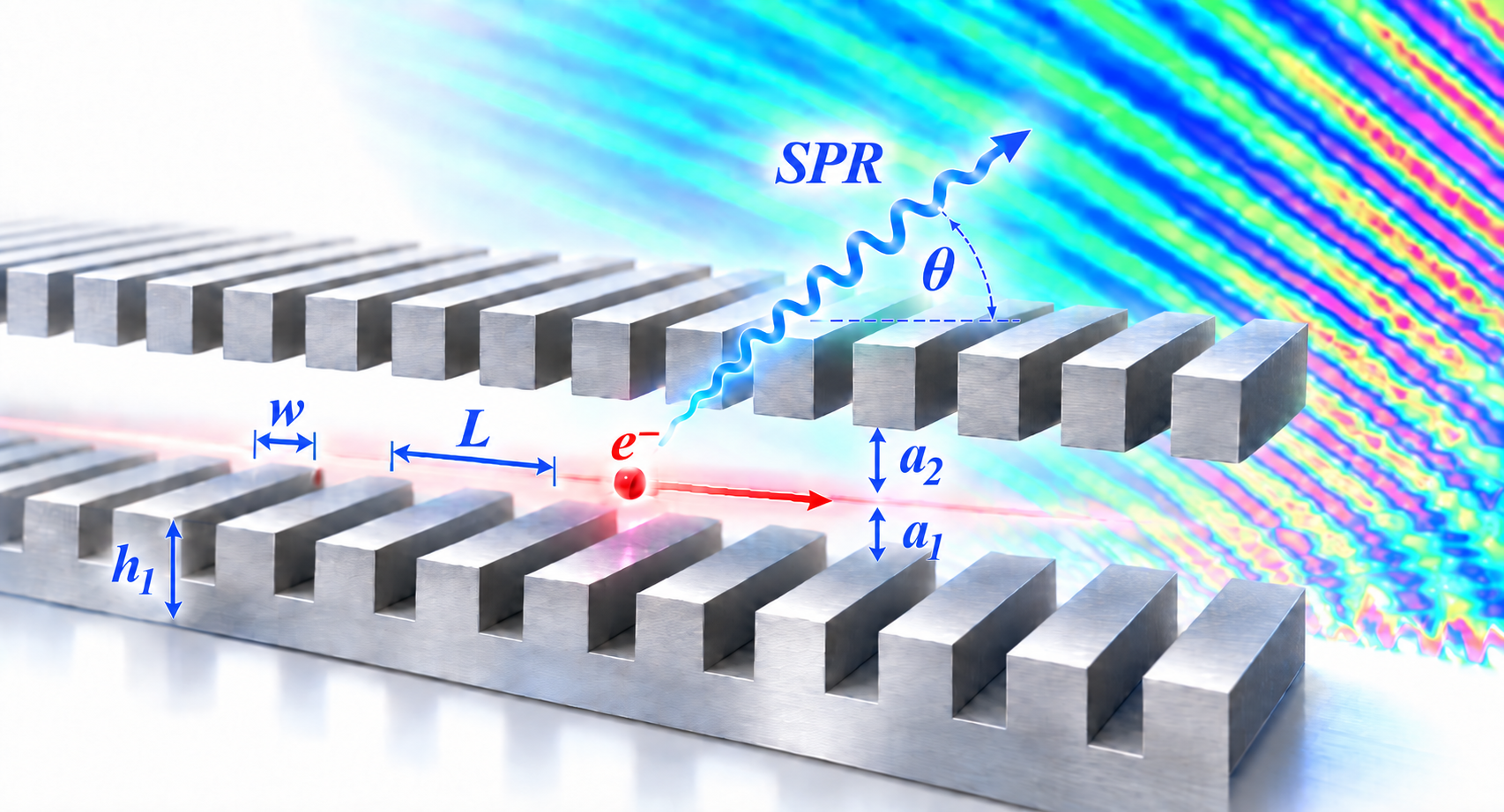
A second layer can help — but only when the physics says it should

A two-layer grating looks like an obvious upgrade to a conventional Smith–Purcell structure: place a second periodic metallic grating on the other side of the electron beam and create a stronger electromagnetic interaction region.

The important result of our 2025 IEEE Transactions on Plasma Science study is that the story is not that simple.

A two-layer grating can strongly enhance coherent Smith–Purcell radiation, increase the spatial growth rate, and reduce the starting current. But the enhancement is not universal. Whether the second layer helps depends on the grating geometry, the electron-beam energy, the operating point on the dispersion curve, and the resulting spatial growth rate.

That leads to a much more useful design question:

For a given beam energy and grating geometry, should the device use one grating layer or two?

The paper develops a physics-based way to answer that question.

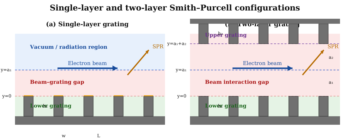
Start with the Smith–Purcell interaction

When an electron beam travels close to a periodic grating, it can excite an evanescent surface wave. The familiar Smith–Purcell wavelength relation is

\[\lambda = \frac{L}{n} \left( \frac{1}{\beta} - \cos\theta \right),\]

where $L$ is the grating period, $n$ is the diffraction order, $\beta=v/c$, and $\theta$ is the radiation angle.

For coherent backward-wave-oscillator-type Smith–Purcell radiation, however, knowing the radiation wavelength is only the beginning. The practical device must also develop enough beam bunching and wave amplification for coherent oscillation to start.

That introduces the starting current: the threshold beam current required to excite sustained coherent radiation.

Reducing this current is valuable because a lower beam current can reduce beam loss, reduce heating of beam-carrying components, and help extend cathode lifetime.

What does the second grating layer actually change?

The second layer changes the electromagnetic boundary conditions seen by the surface mode.

In a single-layer structure, the beam couples to the slow evanescent wave associated with one periodic grating. In the two-layer configuration, the beam is placed between two periodic metallic surfaces. The additional layer changes the allowed electromagnetic modes and therefore changes the grating dispersion.

The consequence is important:

\[\text{grating geometry} \rightarrow \text{dispersion} \rightarrow \text{beam–wave coupling} \rightarrow \text{spatial growth} \rightarrow \text{starting current}.\]

The second layer is useful only when that chain moves the operating point into a region with stronger beam-driven growth.

Step 1 — cold-tube dispersion finds the operating point

The cold-tube problem is solved without dynamic beam loading. It describes the wave propagation supported by the grating structure itself.

For the two-layer grating, the cold-tube model is obtained by solving Maxwell’s equations in the different field regions and enforcing continuity of the tangential field components at the grating interfaces.

The main geometric variables are

\[w,\qquad h_1,\qquad h_2,\qquad a_1,\qquad a_2,\qquad L.\]

Changing these parameters shifts the cold-tube dispersion curve.

The electron beam introduces the beam line

\[\omega = k v_0.\]

Its intersection with the cold-tube dispersion determines the evanescent-wave operating frequency.

For the 50-keV example with

\[w=60~\mu\mathrm{m}, \qquad h_1=h_2=40~\mu\mathrm{m},\]

the calculated evanescent-wave frequencies were approximately

\[f_{\mathrm{ev,1}}=0.717~\mathrm{THz}\]

for the single-layer grating and

\[f_{\mathrm{ev,2}}=0.68~\mathrm{THz}\]

for the two-layer grating.

Because the radiating Smith–Purcell wave occurs at the second harmonic in this configuration, the corresponding theoretical radiation frequencies are about

\[1.43~\mathrm{THz} \quad\text{and}\quad 1.36~\mathrm{THz}.\]

The PIC simulations gave approximately $1.39$ and $1.32~\mathrm{THz}$, respectively. The small shift is consistent with beam loading, space charge, and nonlinear effects that are present in PIC but absent from the passive cold-tube calculation.

This agreement is useful because it shows that the simpler dispersion calculation can locate the operating frequency before a full PIC study is performed.

Step 2 — hot-tube dispersion tells us whether the wave grows

The hot-tube model includes the electron beam.

The field equations are coupled to the beam continuity equation and equation of motion. At a real operating frequency from the cold-tube solution, the hot-tube equation is solved for a complex wavenumber,

\[k = k_r + j k_i.\]

With the field convention used in the paper,

\[E(x,t) \propto e^{-j\omega t+jkx} = e^{-j\omega t} e^{j k_r x} e^{-k_i x}.\]

Therefore,

\[k_i<0\]

corresponds to spatial growth, and the magnitude

\[-k_i\]

is the spatial growth rate.

This is the central design quantity.

A larger spatial growth rate means that the beam-driven mode amplifies more strongly along the interaction length.

Step 3 — spatial growth predicts the starting-current trend

The paper compares the hot-tube spatial growth rate with starting currents obtained independently from PIC simulations.

For the two-layer structure, the same correlation previously identified for single-layer gratings remains clear:

The grating parameters that produce a larger spatial growth rate also produce a lower starting current.

For the 50-keV optimization study, the second-layer height was found to be favorable near

\[h_2=40~\mu\mathrm{m}.\]

With that value fixed, strong growth was obtained when the groove width was approximately

\[w=60\text{–}80~\mu\mathrm{m}\]

and the first-layer height was close to

\[h_1=100~\mu\mathrm{m}.\]

For the reported optimized case,

\[w=60~\mu\mathrm{m}, \qquad h_1=100~\mu\mathrm{m}, \qquad h_2=40~\mu\mathrm{m},\]

the PIC-calculated starting current reached approximately

\[I_s=12.5~\mathrm{A/m}.\]

The same geometry also corresponded to the strongest spatial-growth region in the theoretical calculation.

A dramatic example — but it should not be generalized blindly

One of the clearest PIC examples used

\[w=60~\mu\mathrm{m}, \qquad h_1=h_2=40~\mu\mathrm{m}.\]

At a beam current of $2000~\mathrm{A/m}$, introducing the second grating layer produced approximately a fourfold increase in radiation intensity compared with the single-layer structure.

The two-layer structure could also operate at only $500~\mathrm{A/m}$ while producing a radiation level comparable to the single-layer structure operating at $2000~\mathrm{A/m}$.

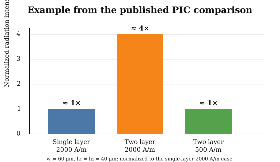
This example shows why the two-layer concept is attractive.

But the more important result of the paper is that the same improvement does not occur everywhere in parameter space.

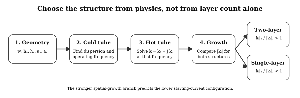
The most useful design rule: compare the growth rates

Let

\[|k_i|_{\mathrm{two}}\]

and

\[|k_i|_{\mathrm{single}}\]

represent the spatial-growth magnitudes for otherwise comparable two-layer and single-layer designs.

The paper shows the following selection rule:

\[\frac{|k_i|_{\mathrm{two}}} {|k_i|_{\mathrm{single}}} >1 \quad \Longrightarrow \quad \text{two-layer structure tends to require lower starting current},\]

while

\[\frac{|k_i|_{\mathrm{two}}} {|k_i|_{\mathrm{single}}} <1 \quad \Longrightarrow \quad \text{single-layer structure tends to require lower starting current}.\]

The PIC starting-current calculations followed this prediction across the tested comparison points.

This is much more useful than assuming that adding another grating automatically improves performance.

Why the upper band edge matters

The calculations show that the strongest spatial growth generally occurs when the beam-synchronous operating point approaches the upper band edge,

\[\bar{k}\approx\pi.\]

This region is particularly susceptible to beam-driven instability.

For some grating dimensions, the two-layer structure shifts the operating point closer to this high-growth region and therefore reduces the starting current.

For other dimensions, the second layer shifts the operating point away from the favorable band-edge region. In those cases, the single-layer configuration can have a higher growth rate and a lower starting current.

That explains why geometry optimization cannot be separated from the choice of one or two layers.

The second layer shifts the useful beam-energy range

A particularly important result appears when the beam energy is varied.

Across the parametric study, the spatial-growth bands of the two-layer structures shift toward lower beam energy compared with the corresponding single-layer structures.

This means that, for many geometries, the two-layer configuration can produce stronger spatial growth at lower beam energies.

At higher beam energy, the situation can reverse and the single-layer structure can have the larger growth rate.

This gives the second layer a practical role:

It provides an additional degree of freedom for moving a strong-growth operating region toward the beam energy available in the device.

The second layer is therefore not simply an enhancement layer. It is a dispersion-engineering tool.

What happens when the upper grating is moved away?

The distance between the beam and the second grating also matters.

As the upper layer is moved far from the electron beam, its electromagnetic influence becomes weak. The calculated two-layer cold-tube dispersion then approaches the single-layer dispersion, and the corresponding spatial-growth bands also begin to overlap.

Physically, this is exactly what should happen:

\[a_2\rightarrow\text{large} \quad\Rightarrow\quad \text{second layer becomes electromagnetically irrelevant}.\]

This limiting behavior provides another useful consistency check for the two-layer theory.

Material conductivity matters too

The idealized dispersion theory is useful for identifying the underlying physics, but a real THz grating is not a perfect conductor.

The paper therefore also used CST PIC simulations to examine the effect of finite grating conductivity.

For both single-layer and two-layer structures, increasing conductivity increased the output power and reduced the starting current.

The physical reason is straightforward: lower-conductivity materials dissipate more electromagnetic energy as Joule heating, leaving less field energy available for beam–wave interaction.

For the tested geometry, the two-layer structure retained a higher output power and lower starting current because it was operating in a parameter region with the stronger spatial-growth rate.

This shows that electromagnetic loss and dispersion optimization have to be considered together in a practical THz source.

A useful workflow for future grating designs

The study suggests a computationally efficient strategy for designing Smith–Purcell structures:

1. Choose candidate values of $w$, $h_1$, $h_2$, $a_1$, $a_2$, and $L$.
2. Solve the cold-tube dispersion.
3. Find the beam-synchronous operating frequency.
4. Solve the hot-tube dispersion for the growing complex root.
5. Map $-k_i$ over the geometry and beam-energy range.
6. Compare the single-layer and two-layer growth rates.
7. Use PIC simulations only for the most promising candidates.
8. Include realistic material conductivity when moving toward a practical device.

This approach is considerably more informative than sweeping starting current by brute-force PIC simulation for every possible geometry.

The broader lesson

The most important idea is not simply that a two-layer grating can produce more radiation.

It is that the number of grating layers changes the dispersion landscape, and the device performance follows from where the beam interacts with that landscape.

For one operating point, the second layer can place the beam near a high-growth branch and dramatically reduce the required current.

For another operating point, the same additional layer can move the system away from the favorable region.

So the design principle is:

Do not choose the number of grating layers first. Choose the operating point first, calculate the spatial growth, and let the beam–wave physics determine the structure.

That principle can be useful not only for Smith–Purcell sources but also for more complicated periodic slow-wave structures used in free-electron radiation devices.

References

1. M. A. Faisal and P. Zhang, “Parametric Analysis on Enhancement of THz Smith–Purcell Radiation by Two-Layer Grating Structure,” IEEE Transactions on Plasma Science, vol. 53, no. 6, pp. 1170–1185, 2025. DOI: 10.1109/TPS.2025.3567163 ↗

2. S. J. Smith and E. M. Purcell, “Visible Light From Localized Surface Charges Moving Across a Grating,” Physical Review, vol. 92, no. 4, p. 1069, 1953. DOI: 10.1103/PhysRev.92.1069 ↗

3. M. A. Faisal and P. Zhang, “Grating Optimization for Smith–Purcell Radiation: Direct Correlation Between Spatial Growth Rate and Starting Current,” IEEE Transactions on Electron Devices, vol. 70, no. 6, pp. 2860–2863, 2023. DOI: 10.1109/TED.2022.3208846 ↗

4. P. Zhang, L. K. Ang, and A. Gover, “Enhancement of Coherent Smith–Purcell Radiation at Terahertz Frequency by Optimized Grating, Prebunched Beams, and Open Cavity,” Physical Review Special Topics – Accelerators and Beams, vol. 18, 020702, 2015. DOI: 10.1103/PhysRevSTAB.18.020702 ↗

5. D. Li et al., “Growth Rate and Start Current in Smith–Purcell Free-Electron Lasers,” Applied Physics Letters, vol. 100, 191101, 2012. DOI: 10.1063/1.4711803 ↗

6. J. P. Verboncoeur, A. B. Langdon, and N. T. Gladd, “An Object-Oriented Electromagnetic PIC Code,” Computer Physics Communications, vol. 87, pp. 199–211, 1995. DOI: 10.1016/0010-4655(94)00173-Y ↗

7. Y. Y. Lau and D. Chernin, “A Review of the AC Space-Charge Effect in Electron–Circuit Interactions,” Physics of Fluids B, vol. 4, no. 11, pp. 3473–3497, 1992. DOI: 10.1063/1.860356 ↗

8. D. M. H. Hung et al., “Absolute Instability Near the Band Edge of Traveling-Wave Amplifiers,” Physical Review Letters, vol. 115, 124801, 2015. DOI: 10.1103/PhysRevLett.115.124801 ↗